Data Science Lab (ECE 460J) - Final Project
Author’s Note: Our fine-tune process in the video was broken, and our analysis has changed! Keep reading…
Introduction
Retrieval-Augmented Generation (RAG) systems are only as good as their retrieval step. Even without powerful language models, poor document retrieval leads to weak, incorrect, or useless outputs. However, evaluating retrieval systems is difficult, and it requires a dataset that clearly defines what the correct document should be for any given query. In this project, we set out to build our own synthetic (question, document) dataset, and use it to evaluate different retrieval methods. Instead of relying on existing benchmarks, we created a pipeline that generates queries from real documents and measures how well the different models retrieve the correct information.
What We Did
Our goal was to simulate a real-world retrieval problem: Given a query about supreme court cases, which retrieval method is most effective at finding the correct case? To answer this question, we:
- Built a dataset of (question, documents) pairs
- Fine-tuned our own embedding model on our data set
- Compared multiple retrieval methods (TF-IDF, BM25, embedding models) using ranking metrics (recall, precision, ndcg)
- Analyzed the results
Scraping the Data
We were interested in coming up with our own data set. To keep things interesting (but not too difficult), we decided on scraping summaries of US Supreme Court from Oyez.org. Each case summarized by Oyez usually comes with a summary of the case and a conclusion, which are usually about the size of a paragraph. Each page is also homogenous, which greatly simplifies data set creation.
Selenium is a natural choice for scraping, but it is a bit heavy. It’s always worth checking if your page fetches data from an API. Many times, you can leverage this for scraping purposes. Usually, this only involves opening up your browser’s developer tools and poking around in the “Network” tab.
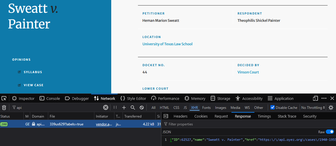
Discovering the Oyez API
Lucky for us, we can see that Oyez has an API we can use, which saves a fair bit of work parsing out the data ourselves. In order to scrape every case, we need to first scrape the listing. The requests library makes this relatively easy:
BASE_URL = "https://api.oyez.org"

session = requests.Session()
session.headers.update({
    "User-Agent": "OyezResearchScraper/1.0 (Academic)", # It's polite to be honest with your user agent
    "Accept":     "application/json",
})

all_cases = []
while True:
    r = session.get(f"{BASE_URL}/cases", params={"per_page": PER_PAGE, "page": page})
    data = r.json()
    if not data:
        break
    all_cases.extend(data)
    if len(data) < PER_PAGE:
        break
    page += 1
This gives us a bunch of stubs that look like this:
[
    {
        "ID": 49051,
        "name": "American Trucking Assns., Inc. v. United States",
        "href": "https://api.oyez.org/cases/1966/510",
        ...
    },
    ...
]
We can fetch all of the more in-depth case details by querying the href fields provided in each stub. The code to do this is very similar to the above. Once we have the stub and the detailed information for each case, we can flatten it down into a simple list of records:
def flatten(stub, detail):
    dec             = (detail.get("decisions") or [{}])[0]
    decision_raw    = dec.get("decision_type") or {}
    disposition     = disposition_raw.get("label", "") if isinstance(disposition_raw, dict) else str(disposition_raw)
    decision_type   = decision_raw.get("label",   "") if isinstance(decision_raw,   dict) else str(decision_raw)

    # Term & docket (prefer detail, fall back to stub)
    term   = str(detail.get("term")          or stub.get("term")          or "")
    docket = str(detail.get("docket_number") or stub.get("docket_number") or "")

    return {
        "term":           term,
        "docket_number":  docket,
        "oyez_id":        str(detail.get("ID") or detail.get("id") or ""),
        "name":           (detail.get("name") or stub.get("name") or "").strip(),
        "citation":       detail.get("citation") or "",
        "first_party":    (detail.get("first_party") or "").strip(),
        "second_party":   (detail.get("second_party") or "").strip(),
        "winning_party":  dec.get("winning_party") or "",
        "disposition":    dec.get("disposition") or {},
        "decision_type":  decision_type,
        "majority_vote":  dec.get("majority_vote"),
        "minority_vote":  dec.get("minority_vote"),
        "facts_of_the_case":  (detail.get("facts_of_the_case")  or "").strip(),
        "question":       (detail.get("question")       or "").strip(),
        "conclusion":     (detail.get("conclusion")     or "").strip(),
        "href":           detail.get("href") or stub.get("href") or "",
    }


records = []
for stub, detail in case_data:
    records.append(flatten(stub, detail))
Here, we mostly care about the facts_of_the_case and conclusion fields, which contain the actual summaries of each supreme court case. We retain the other data just in case we need it.
Of course, at this point, it’s convenient to convert our data into a pandas DataFrame, which makes interacting with our data much more convenient:
df = pd.DataFrame(records).set_index("oyez_id")
That’s really all there was to scraping here: just parsing JSON from a bunch of API endpoints! But we still have to do…
Dataset Construction
Naturally, our data has some imperfections, including duplicates, and some raw HTML we need to rid ourselves of. Somehow, during the scraping process we found that some cases got scraped many times—no good. Luckily, since we index on the unique id for each case, we can use an elegant pandas one-liner, which will collapse all of our duplicate entries by unique id:
df = df.groupby(df.index).agg('first') # This dropped 70 duplicate entries!
We’re also primarily interested in the text content of these pages, so any rows without any text content are useless to us. Doing this is a bit ugly in pandas; we can find all the row indexes that do have at least one text field filled, then regenerate our DataFrame. It’s not efficient, but it gets the job done:
content_columns = ['facts_of_the_case', 'question', 'conclusion'] # Columns with our text content
df = df[~df[content_columns].isna().all(axis=1)]                  # Drop rows where all content is empty
This dropped 4666 rows, leaving only 3746! It seems Oyez has a backlog…
Another slight kink is that our dataset text is formatted in HTML. Luckily, BeautifulSoup makes parsing out HTML very easy. While we’re at it, we can strip out non-breaking space characters and newlines:
from bs4 import BeautifulSoup

for oyez_id in df.index:                                          # Iterate over all oyez_ids
    for field in ['facts_of_the_case', 'question', 'conclusion']: # Each over our text columns
        text_body = df.loc[oyez_id][field]
        if isinstance(text_body, str):                            # Skip nan fields
            soup = BeautifulSoup(text_body, 'html.parser')

            # This will extract the text (without HTML tags)
            text_content = soup.text.replace(u'\xa0', ' ').replace("\n", " ")
            df.loc[oyez_id, field] = text_content
Interestingly, some pages had non-empty text fields that were only filled with blank space. Best we filter that out too. We can do this by regenerating each text-column, setting it to nan if it has fewer than 25 characters. Since this may produce more rows with no valid text data, we need to repeat our little trick to drop those rows:
content_columns = ['facts_of_the_case', 'question', 'conclusion'] # Columns with our text content
df[content_columns] = df[content_columns].apply(
    lambda col: col.where(col.str.len().fillna(0).ge(25), other=np.nan) # nan-ify anything shorter than 25 chars
)
df = df[~df[content_columns].isna().all(axis=1)] # Drop rows where all content is empty
And, of course, with all this work done, we save our data:
df.to_csv(CSV_OUTPUT)
Generating a Data Set
To try to evaluate different options for retrieval, we need to turn this scraped data into a set of questions and relevant documents. Even better, we can make our data richer by ranking how relevant each document is with respect to each question.
However, this poses a slight problem: manually generating questions from over 3,000 documents is time-consuming and requires significant mental effort. Luckily, modern LLMs can help out here; cheap models can generate our data set for just a few dollars. However, we still need to be smart about how we leverage LLMs. Since we want questions that target similar documents, we can try using a large embedding model to group like cases together. That way, we can feed a small selection of documents to an LLM, which will keep things cheap (and possible!):
from openai import OpenAI

client = OpenAI(api_key=OPENAI_API_KEY)

def get_embeddings(queries):
    embeddings_arr=[]
    for query in batched(queries, 10):
        embeds = client.embeddings.create(
            model="text-embedding-3-large",
            input=query,
            encoding_format="float"
        )
        for result in embeds:
            embeddings_arr.append(result.embedding[0])
    return embeddings_arr

# Need to cast nans to actual text values. We're too lazy to skip over them :P
facts_arr = df['facts_of_the_case'].fillna('Unknown').to_list()
conclusion_arr = df['conclusion'].fillna('Unknown').to_list()

embeddings_facts = get_embeddings(facts_arr)
embeddings_conclusion = get_embeddings(conclusion_arr)
df['facts_openai'] = embeddings_facts
df['conclusion_openai'] = embeddings_conclusion
This generates 3,072-dimensional embedding vectors that encode the semantic meaning of each of our chunks. At this point, we need to save our data again. This time, we’ll use the parquet format, since CSV won’t store these new 11.5 million numbers very efficiently.
df.to_parquet("oyez_cases_embeddings_openai.parquet") # About 80 MB vs 180 MB with CSV!
With some luck, similar vectors will correspond to potentially related supreme court cases. K-Means clustering allows us to find which of these vectors are near each other. Of course, we do this for both the facts_of_the_case fields and conclusion text fields:
from sklearn.cluster import KMeans
import numpy as np

embeddings_facts = np.vstack(df['facts_openai'].to_numpy())

# Find clusters
facts_clusters = KMeans(
    n_clusters=(len(embeddings_facts)//10),
    random_state=0, n_init="auto"
).fit(embeddings_facts)

# Generate a mapping of cluster number -> index in embeddings_facts
facts_index_map = {
    val: np.where(facts_clusters.labels_ == val)[0] for val in np.unique(facts_clusters.labels_)
}
The index map gives us a bunch of chunks that are clustered together that look like this:
0: [ 415, 1763,  ..., 3682]
1: [  38,   87,  ..., 2995]
2: [ 145,  404,  ..., 3213]
For fun, we can pick a cluster and see if we can spot why they may have clustered together. We’ll take the cluster [440, 627] and look them up:
440_facts: "The city of Pawtucket, Rhode Island, annually erected a Christmas display located in the city's shopping district. The display included..."
627_facts: "Two public-sponsored holiday displays in Pittsburgh, Pennsylvania, were challenged by the American Civil Liberties Union. The first display..."
It’s easy to see how these are related—they’re about holiday displays! Fortunately, most clusters we manually inspected shared similarities like this, which is a great sign that our clustering was successful!
LLMs to the Rescue
Now that we have clusters we can feed to an LLM, we need to figure out how to get the LLM to generate the data we want. A good start is coming up with a system prompt that commands it to do our bidding. In our case, we want three questions per cluster. It would also be helpful if we knew what chunks are relevant to each question, so we can ask it to rank the relevance of each chunk for each generated question. Also, if there are any documents not related to the generated question, we could keep them around as hard-negative candidates, since they were similar enough to be clustered.
Importantly, writing a good system prompt can make a huge difference in the outcome, so it’s worth spending some time on. For instance, we were getting a lot of questions that included actual statute numbers, which was certainly too specific. Prompting to avoid legal jargon seemed to help mitigate that issue. Here’s what we ultimately came up with:
Given summaries of supreme court cases, generate three realistic questions that an average person would ask such that the answer is best found in this chunk. You MUST pretend that you do not know what the correct case or specifics are when formulating the question (i.e., it should be a question with an unknown document for an answer; the idea is that this is used to train a RAG to find it for us). Limit the number of questions that include the case name or a person name to 2 or three max. Avoid using legal jargon like specific case law; keep questions simple and general enough. Document ranks must be distinct (i.e., no two documents can be ranked the same for a given question). Determine if each of the supplied cases is relevant to the question, rank its relevance, and give a short reason as to the ranking. Ensure there is only ONE document per oyez_id (i.e., no duplicate ids)!
Of course, we need to generate the prompts that we’ll use when we feed each cluster into the LLM. Since we’ve already given the LLM instructions in the system prompt, we can just give it the clustered case chunks. A little helper function is all we need to do this:
def build_prompt(clustered_chunks, field='facts_of_the_case'):
    prompt = ""
    for ind in clustered_chunks:
        row = df.iloc[ind] # Clustered chunk ids are indices onto our dataframe
        prompt += f"{row['name']} (OYEZ ID: {row.name}) \n{row[field]}\n\n"
    return prompt
Which gives us prompts that look like:
American National Red Cross v. S.G. (OYEZ ID: 54039)
Plaintiffs filed two state-law tort actions in New Hampshire state courts...

Correctional Services Corporation v. Malesko (OYEZ ID: 54999)
In 1993, John E. Malesko was assigned to a bedroom...

Nevada Department of Human Resources v. Hibbs (OYEZ ID: 55104)
William Hibbs, an employee of the Nevada Department of Human Resources, sought leave...

Frew v. Hawkins (OYEZ ID: 55134)
In 1996, Linda Frew and other citizens settled...
However, even with our prompts prepared, we still need to address the issue of what we’re going to do with the LLM’s response. You may notice that we haven’t specified an output format in our prompt. This is intentional, because we’re going to use a convenient thing called structured output!
Structured Output
Modern LLM APIs allow us to enforce a schema for our response, which makes parsing it a piece of cake. In Python, your favorite LLM bindings probably support structured output using pydantic. Pydantic makes parsing data into complex nested structures very easy. Aside from being useful in many data-parsing contexts, it can also be used to generate schemas for our LLM! All we have to do is define our response as a set of models:
from pydantic import BaseModel

# A related document, relevance rank, reason, etc.
class RelatedDocument(BaseModel):
    oyez_id: int
    chunk_type: Optional[ChunkType] = None
    relevance: RelevanceClass
    relevance_rank: int = Field(description="How relevant the document is. Must be unique")
    reasoning: str = Field(description="Why the document is relevant")

# A question and its associated relevant/irrelevant documents
class GeneratedQuery(BaseModel):
    question: str = Field(description="A natural realistic question from a real person...")
    docs: list[RelatedDocument] = Field(description="Relevant documents. There must be EXACTLY one document per oyez_id, no more, no less")

# A collection of questions from the LLM
class QueryBatch(BaseModel):
    queries: list[GeneratedQuery]
Finally, we can send it off to our LLM and get our response in our desired (and parsed) format!
gpt_response = client.responses.parse(
    model="gpt-5-mini",
    input=[
        {"role": "system", "content": SYSTEM_PROMPT},
        {
            "role": "user",
            "content": build_prompt(facts_index_map[321]),
        },
    ],
    reasoning={"effort": "medium"},
    text_format=QueryBatch,
) # Will return an instance of QueryBatch :D
LLM Batching
It’s worth noting that, since we’re working with lots of prompts, most LLM providers offer batch systems. The idea is that you upload tons of prompts that don’t need immediate processing. In exchange for possibly waiting a day for your results, you get a discount on usage (usually about half off!). With this in mind, we don’t actually make the requests ourselves. Instead, we generate a big .json file with all of our prompts (and the schema of course). We take this file and upload it straight to OpenAI for processing with gpt-5-nano. We then download the results (which are just a .jsonl), and parse them into our pydantic schemas. The details of how we generate batches are in the embeddings.ipynb file in the GitHub repo. The biggest hurdle is that we have to dump our pydantic schemas into something the batch API likes. The broad strokes are the same, it’s just a bit too technical to discuss here.
Validating the LLM Output
Unfortunately, using structured outputs with an LLM does not guarantee any stability with the generated data; it only (mostly) guarantees that it will be in a parsable format. Therefore, we need to screen the LLM’s work for basic mistakes. Luckily, the questions themselves are easy enough to review by hand. Still, we can scan each returned question-documents pair for issues, including listing chunks multiple times, ranking two chunks the same (we asked it not to), hallucinating a chunk id, not giving a relevance rank to all chunks, and so on. The code for this is in the repository; it’s not very interesting.
Pydantic’s model_validators seemed like a great fit for this, and we did (unfortunately) use them. The idea is that you can raise an error if you ever try to manipulate your pydantic model in a way you shouldn’t. For instance, if I parse an LLM response that ranks two chunks the same, then I can raise an error. Optionally, model validators can also edit the data too, which is helpful for imputing missing chunk ranks (i.e., if any chunks aren’t listed, we rank them last). However, this does not play very nicely with LLM bindings in Python, since most bindings will try to be helpful and parse the output into your model. If you need to pass additional context to the model validator (which we do), this significantly complicates things. You essentially have to hack in an on-switch for your validators; if the validator fails, your entire LLM response could get blown-up by the raised exception. It’s just way too clunky when you can just manually validate it outside of using a model_validator. Still, validators are worth knowing about if you ever use pydantic for a different project.
class GeneratedQuery(BaseModel):
    ...

    @model_validator(mode="after")
    def validate_unique_relevance_ranks(self, info: ValidationInfo) -> GeneratedQuery:
        # Checks if relevance ranks are unique, raises error if not
        ...
Finally, after all that trouble, we get question-document pairs that look like this:
{
  "question": "If a state tort case about a tainted blood transfusion is moved to federal court by the defendant under a removal statute, can the federal court keep it there or must it be remanded back to state court?",
  "docs": [
    {
      "oyez_id": 54039,
      "chunk_type": "facts",
      "relevance": "relevant",
      "relevance_rank": 1,
      "reasoning": "Addresses the key issue of removal from...",
      "chunk_id": "54039_facts"
    },
    ...,
    {
      "oyez_id": 63419,
      "chunk_type": "facts",
      "relevance": "irrelevant",
      "relevance_rank": 9,
      "reasoning": "Omitted by LLM",
      "chunk_id": "63419_facts"
    }
  ]
}
Methods and Models
After building the dataset, we want to figure out what retrieval methods are effective at finding the correct document for our queries. These methods fell into two main categories: lexical retrieval and dense embedding retrieval.
The two lexical methods we’re interested in are BM25 and TF-IDF. In short, TF-IDF tries to score document relevance based on how often a word from the query appears in the search documents. The idea is that, for each word in the query, if lots of documents have that word, it’s probably not super indicative of document relevance. By contrast, if a query word appears in just a few documents, it probably tells us a lot about the document’s relevance. BM25 is similar, but it also has a few enhancements. BM25 adds diminishing returns to search term frequency, which mitigates an issue in TF-IDF called term frequency saturation. When TF-IDF ranks documents, it may prefer documents that repeat a query word many times, even if the document isn’t truly any more relevant. By contrast, BM25 tempers preference for documents that frequently use a query term. It also normalizes for document length, which makes rankings more “fair” amongst documents with a wide range of lengths. Importantly, these models only care about exact keywords. They don’t account for synonyms or contextual meaning. Still, we’ll later see they perform quite well on our data set.
We also tested dense embedding models using SentenceTransformers. Embedding models differ from lexical methods in the sense that they try to extract meaning from the query. To do this, these models convert queries and documents into vectors, then rank documents based on how similar their vectors are to a query vector. Embedding-based retrieval is useful because it can capture semantic similarity even when the query and document do not use the exact same wording. However, these models are usually more computationally expensive than lexical methods, especially considering larger models like Qwen3-Embedding-4B.
Here’s the shortlist of off-the-shelf models we want to investigate:
- MiniLM
- BGE
- BERTUncased
- Qwen3-0.6B
- Qwen3-4B
A Brief Attempt at Training
In addition to our off-the-shelf models, we may also want to see how a specially trained model performs on our data. For this project, we’ll give tuning MiniLM a shot. In theory, sentence-transformers should make this a breeze.
To do this, we need to convert our synthetic dataset into a format that SentenceTransformers can consume. Since each query in our dataset was paired with ranked relevant documents, we could transform these examples into training pairs where the model learns which documents should be closer to a query in embedding space. All we are really doing is generating pairs of (query, most_relevant_document):
def flatten_entry(entry):
    # Ensure all of our query positives are sorted by rank properly
    positives = sorted(
        [d for d in entry["docs"] if d["relevance"] == "relevant"],
        key=lambda d: d["relevance_rank"]
    )

    # Including negatives actually hurt our validation scores a bit!
    rows = []
    if positives:
        rows.append({
            "query": entry["question"],
            "positive": id_text_map[positives[0]["chunk_id"]],
        })

    return rows

# Load the (query, chunks) dataset
with open("../api/improved_dataset2.jsonl", "r", encoding="utf-8") as f:
    query_objs = [json.loads(x) for x in f.readlines()]

# Split off 200 of the 2123 questions to use for evaluation
eval_queries = query_objs[:200]
train_queries = query_objs[200:]

eval_dataset = []
for obj in eval_queries:
    for datapoint in flatten_entry(obj):
        eval_dataset.append(datapoint)

train_dataset = []
for obj in train_queries:
    for datapoint in flatten_entry(obj):
        train_dataset.append(datapoint)

eval_dataset = Dataset.from_list(eval_dataset)
train_dataset = Dataset.from_list(train_dataset)
We experimented with including hard negatives when generating these pairings, but it actually marginally hurt performance. This could mean our lazy way of mining hard negatives wasn’t very effective. Nevertheless, not having hard negatives is not an issue, since we’ll be able to use the other documents in the batch as negatives. Now, all we need to do is train:
model = SentenceTransformer("sentence-transformers/all-MiniLM-L6-v2")

loss = MultipleNegativesRankingLoss(model) # uses InfoNCE under the hood

args = SentenceTransformerTrainingArguments(
    output_dir="output/minilm-finetune-fixedeval-mnrl",
    num_train_epochs=3,
    per_device_train_batch_size=64, # Large enough batches for InfoNCE to work well
    learning_rate=2e-5,
    warmup_ratio=0.1,
    eval_steps=500,
    eval_strategy="steps",
    save_strategy="steps",
    save_steps=500,
    load_best_model_at_end=True,
)

trainer = SentenceTransformerTrainer(
    model=model,
    args=args,
    train_dataset=train_dataset,
    eval_dataset=eval_dataset,
    loss=loss
)

trainer.train()

model.save_pretrained("output/minilm-finetune")
As an aside, we tried using MarginMSELoss for this, since we could have (query, positive, negative, label) pairs, where label was how “negative” the example was. After finetuning, we saw that our training loss got better. However, on our holdout set, loss did not improve at all, so we weren’t actually making any improvement. We think there are a few reasons for this. Primarily, when we used this method, we made a training pair for every positive document and all corresponding negative combinations. It is also likely our per_device_train_batch_size was too small. Good thing we were able to fix it by using MultipleNegativesRankingLoss and increasing our batch sizes.
Evaluating Our Options
Now that we have a bunch of off-the-shelf models and our own fancy fine-tuned model, we need to benchmark them. To do this, we’ll need to use a few different metrics to see how each option performs. Generally, when we’re searching, we’re only going to consider some of the top returned documents. We may think of this as a “first page on a Google search”—we usually aren’t interested in anything more than the top results. We’ll call the number of top results we retrieve K. When we talk about some Metric@K, what we mean to say is that we’re evaluating that metric if we just look at our top K documents. There are three common metrics that we’ll look at today:
Recall@K: Recall tells us how many of the relevant documents were returned for some query. For example, if we got one relevant document, but we could’ve gotten ten relevant documents, our score would be
0.1. We might think of this metric as how “comprehensive” our top-k is. Importantly, this metric does not care about how relevant documents are or how they are ranked, only if they are relevant.Precision@K: Precision tells us what fraction of our top-k documents are relevant. For instance, if all of our
kdocuments are relevant, our score would be1. Conversely, we may think of this score as going down as irrelevant documents are included in our top-k. To give an extreme example, if there is only one relevant document and our K is 10, retrieving that document would make ourprecision = 0.1; all of the other 9 results were irrelevant. This also means that as K grows, precision tends to drop naturally, since we are pulling in more results alongside a fixed number of relevant ones. Again, this metric only cares about if a document is relevant, much like Recall@K.NDCG@K (Normalized Discounted Cumulative Gain): This tells us how well our retrieved documents are ordered. Essentially, we want our most relevant documents to come earlier in our top-k documents. The better our list of “top hits” is, the better our NDCG score. Conversely, if our best documents are ranked later in our top-k, our NDCG suffers. The “discounted” part of the name refers to the fact that each position in the ranking is penalized by a logarithmic factor. For instance, a highly relevant document at rank five contributes much less to the score than if it were at rank one. NDCG is a bit flexible in that you can assign relevance scores to each relevant document. Since we had our LLM rank the relevant documents per query, we simply assign
relevance = 1 / rank, which means our NDCG scores will also encode how well our retrieval matched the LLM’s ranking.
With our metrics defined, we can now look at how each retrieval method actually performed. After evaluating each retrieval method on a holdout set of 200 queries (i.e., what our fine-tune did not train on), we get these results for K=10.
| Metric | qwen3-4b | MiniLM-Finetune | BM25 (Okapi) | qwen3-0.6b | bge-small-en-v1.5 | TF-IDF | all-MiniLM-L6-v2 | bert-base-uncased |
|---|---|---|---|---|---|---|---|---|
| Recall | 0.644 | 0.615 | 0.596 | 0.579 | 0.466 | 0.465 | 0.430 | 0.192 |
| Precision | 0.141 | 0.134 | 0.124 | 0.124 | 0.099 | 0.095 | 0.093 | 0.038 |
| NDCG | 0.568 | 0.551 | 0.542 | 0.534 | 0.396 | 0.393 | 0.347 | 0.141 |
K = 10, sorted from best to worst Recall
Qwen3-4b leads with a Recall of 0.644, meaning it found the correct chunk in its top 10 results about 64% of the time. This is a bit lackluster for our purpose, but it is still quite good compared to our other options. Notably, our fine-tuned MiniLM is vastly improved over the base model, achieving an approximate 0.2 increase in Recall and NDCG! BM25 and qwen3-0.6b follow closely behind, with BGE, TF-IDF, and MiniLM firmly performing worse in all metrics. We can also see that precision scores are somewhat low, which is expected, since many of our queries had just a few relevant documents. Lastly, BERT base does poorly, since it’s not trained for retrieval.
Perhaps the most surprising result is how competitive BM25 is. Despite having no intrinsic understanding of language or meaning, it matches or beats most other options on every metric. This is especially clear if we look at the results for K=1. In this case, BM25 actually beats every other option in Precision and NDCG, and is practically tied with Qwen3-0.6b in Recall.
| Metric | qwen3-4b | MiniLM-Finetune | BM25 (Okapi) | qwen3-0.6b | bge-small-en-v1.5 | TF-IDF | all-MiniLM-L6-v2 | bert-base-uncased |
|---|---|---|---|---|---|---|---|---|
| Recall | 0.278 | 0.286 | 0.295 | 0.296 | 0.192 | 0.179 | 0.151 | 0.065 |
| Precision | 0.475 | 0.490 | 0.520 | 0.500 | 0.335 | 0.315 | 0.275 | 0.105 |
| NDCG | 0.431 | 0.453 | 0.464 | 0.446 | 0.302 | 0.287 | 0.236 | 0.092 |
K = 1, in the same order as above
We can see that BM25 ranked a relevant document first more than half of the time—not bad. Of course, we still see a similar trend of the Qwen models, our finetune, and BM25 performing quite well, while the others trail. Since our K is just 1, we lose some granularity in our results, so we see that our four top-performing options are approximately tied in most metrics.
It is also worth noting that our dataset generation method likely contributed to BM25’s success. Since we generated questions from the case summaries using an LLM, it is possible it borrowed the language and exact wording from those documents, giving an unfair advantage to BM25 and TF-IDF. If we built our dataset by gathering relevant cases from a question, rather than generating questions from cases, we may get more realistic results. This limitation is one to be kept in mind for future testing and while interpreting these results.
Conclusions
So if we were building a RAG using Supreme Court cases, what model would we want to use? If we were only concerned with our benchmark scores, Qwen3-4b would be the best choice. However, running a 4-billion parameter model is quite expensive, and we can see that it doesn’t have a significant edge over our MiniLM finetune or BM25. That realistically leaves our finetune as one of the strongest embedding models, so we’d be choosing between BM25 and our finetune. BM25 is without a doubt less computationally expensive to run, with the caveat that our dataset generation may have biased BM25’s performance. Realistically, since embedding models are less sensitive to exact keyword matches, and our finetune performs about as well as BM25, we’d probably want to use the finetune.
It’s also worth considering if our dataset method scales. Of course, it depends. We spent about $1.20 to generate a set of ~370 questions for our ~3700 chunks, which were about 300-500 words each. If we take Wikipedia pages as an example—which are about 700 words on average (source)—then we could likely process about 2000 Wikipedia pages. For a domain-specific use case, this likely isn’t unreasonable; $100 would net you a dataset of about 200,000 queries. You may not even need to go so far to make an effective retrieval system; we were able to get significant improvements with MiniLM on our relatively small data set. Furthermore, the LLM generally only picked a few documents from each cluster to generate documents from. We could trim larger clusters down so each LLM call costs less, at the cost of some negatives. After all, our MiniLM finetune actually did worse with hard negatives, so it may be better to focus on generating more queries instead of lazily mining for negatives.
We hope you learned something, and thanks for reading!